Simulation-based inference

in gravitational wave data analysis

Jacopo Tissino

2026-04-24

The gravitational wave inference problem

What kind of data do we have?

Strain data for the GW250114 event (Abac et al. 2025).

Strain data

\[ d_i = n(i \Delta t) + h(i \Delta t; \theta, M) \]

where typically \(1/\Delta t \approx \text{a few kHz}\).

The contributions are:

• instrumental noise \(n(t)\);
• gravitational wave signal \(h(t; \theta, M)\), which we obtain based on a model \(M\) with parameters \(\theta\).

Stationary Gaussian noise model

Typical assumptions about the noise:

• \(\mathbb{E}[n(t)] = 0\),
• \(\mathbb{E}[n(t) n(t + \Delta t)] = \gamma (\Delta t)\),
• \(\lbrace n(t_1), \dots, n(t_N) \rbrace\) is an \(N\)-dimensional Gaussian random variable for any choice of times \(t_1 \dots t_N\).

Glitches

Examples of glitches in gravitational wave data (Powell 2018).

Gravitational wave likelihood

In full generality:

\[ \mathcal{L}(d | \theta, M) = p(\text{noise realization } n = d - h(\theta, M) | \theta, M) \]

With Gaussian stationary noise:

\[ \mathcal{L}(d | \theta, M) \propto \exp\left( - \frac{1}{2} \int_{f_\text{min}}^{f_\text{max}} \frac{|\tilde{d}(f) - \tilde{h}(f; \theta, M)|^2}{S_n(f)} \text{d} f \right) \]

Bayesian inference

\[ \underbrace{\mathcal{L}(d | \theta, M) \pi (\theta | M)}_{\text{assumptions}} = \underbrace{p(\theta | d, M) \mathcal{Z}(d | M)}_{\text{result}} \]

Figure 1: Posterior distribution on the component masses of GW250114. Adapted from Abac et al. (2025).

Model parameters

The signal parameters \(\theta\) include:

• where is the source in the sky? how is it oriented?
• what masses do the two objects have?
• how fast are they rotating, and in which direction?
• …

Depending on the model, there can be 10–17 parameters.

Simulation-based inference

Simulating from the likelihood

In standard inference, we evaluate the likelihood \(\mathcal{L}(d | \theta, M)\).

In simulation-based inference, we simulate data distributed according to the likelihood:

\[ d \sim \mathcal{L} ( d | \theta, M) \]

Flavors of SBI

• Neural posterior estimation: a density estimator \(q(\theta | d)\) models the posterior \(p(\theta | d)\);
• Neural likelihood estimation: a density estimator \(q(d | \theta)\) models the likelihood (requires sampling);
• Neural ratio estimation: a classifier \(r(\theta, d)\) models the likelihood-to-evidence ratio \(\mathcal{L}(d|\theta) / \mathcal{Z}(d)\) (requires sampling).
• …

More details: Liang & Wang (2025).

Neural posterior estimation in a nutshell

Take a density estimator \(q_\phi (\theta | d)\) with parameters \(\phi\). Train it with a loss function in the form (Dax et al. 2021, Papamakarios & Murray 2016)

\[ L(\phi) = \mathbb{E}_{\theta \sim \pi(\theta)} \mathbb{E}_{d \sim p(d|\theta)} [-\log q_\phi(\theta|d)]\,. \]

If training is successful, the estimator \(q_{\bar{\phi}}(\theta | d)\) at \(\bar{\phi} = \text{argmin}_\phi L(\phi)\) will approximate \(p(\theta | d)\).

Proof

Consider the KL divergence from posterior \(p\) to the estimator \(q\):

\[ D_{\text{KL}}( p || q_\phi) = \int p(\theta | d) \left[ \log p(\theta | d) - \log q_\phi (\theta | d) \right] \text{d}\theta \]

We use as a loss the average over all realizations of the data \(d\):

\[ \begin{aligned} L(\phi) &= \mathbb{E}_{d \sim \mathcal{Z}(d)} [D_{\text{KL}}( p || q_\phi)] \\ &= \int p(\theta | d) \mathcal{Z}(d) \left[ - \log q_\phi (\theta | d) \right] \text{d}\theta \text{d}d + C \end{aligned} \]

Proof

By Bayes’ theorem, \(p(\theta | d) \mathcal{Z}(d) = \mathcal{L}(d | \theta ) \pi(\theta)\), so this is equal to

\[ \begin{aligned} L(\phi) &= \int \pi(\theta) \mathcal{L}(d|\theta) \left[ - \log q_\phi (\theta | d) \right] \text{d}d \text{d}\theta + C \\ &= \mathbb{E}_{\theta \sim \pi(\theta)} \mathbb{E}_{d \sim \mathcal{L}(d|\theta)} \left[ - \log q_\phi (\theta | d) \right] + C \end{aligned} \]

We can compute the expectation value by

• sampling \(\theta\) from the prior \(\pi (\theta)\),
• simulating the data \(d\) from the likelihood \(\mathcal{L}(d | \theta )\).

Normalizing flows

A normalizing flow is an invertible, differentiable map \(T_\phi\) from a simple (e.g. Gaussian) probability distribution \(g(u)\) to an arbitrary one, \(q (\theta)\), so that

\[ u \sim g(u) \iff T(u) = \theta \sim q(\theta) \]

It is often constructed by composing several simple parametric transformations:

\[ T_\phi = T_1 \circ \dots \circ T_N\,. \]

Normalizing flows

To obtain samples from \(q\):

• sample \(u\) from \(g(u)\);
• compute \(\theta = T(u)\);
• we also get the density function as

\[ q(\theta) = g (T_\phi^{-1}(\theta)) |\det J_{T_\phi^{-1}}(\theta)| \]

Toy model: nested sampling versus neural posterior estimation

Problem setup

The example is borrowed from the LAMPE documentation.

Suppose we have a model with three parameters: \(\theta \sim \pi(\theta) = \mathcal{U}([-1, 1]^3)\).

Our data is one observation of

\[ x = \begin{pmatrix} \theta_1 + \theta_2 \theta_3 \\ \theta_1 \theta_2 + \theta_3 \end{pmatrix} + \varepsilon \]

where \(\varepsilon \sim \mathcal{N}^2(\mu = 0; \sigma = 0.05)\).

Standard approach: Nested Sampling

def forward_model(theta):
  return np.array([
    theta[0] + theta[1] * theta[2],
    theta[0] * theta[1] + theta[2]
  ])

def log_like(theta):
    x = forward_model(theta)
    return (
    - 0.5 * ((x-x_obs)**2).sum() 
    / sigma_y**2 + lnorm)

def prior_transform(u):
    return u*2. - 1.

We can then sample with DYNESTY.

New approach: NPE

estimator = NPE(*args, **kwargs)
loss = NPELoss(estimator)
loader = JointLoader(prior, simulator)

optimizer = optim.Adam(
  estimator.parameters())
step = GDStep(optimizer)

for epoch in range(16):
  losses = []
  for theta, x in islice(loader, 256):
      losses.append(
        step(loss(theta, x)))

samples = (estimator.flow(x_obs)
  .sample((2**16,))
)

Validating NPE results

If the likelihood is tractable, we can compute

\[ w_i = \frac{\mathcal{L}(d |\theta_i) \pi(\theta_i)}{q(\theta_i | d)}\,. \]

• We get the evidence as \(Z(d) \approx \langle w_i \rangle\);
• the weighted samples \((\theta_i, w_i)\) are a better representation of the posterior than \(\theta_i\) alone.

Validating NPE results

def effective_samples(samples):

    log_like_times_prior = [
        log_like(sample) + log_prior(sample)
        for sample in samples
    ]

    log_weights = log_like_times_prior - flow_density.detach().numpy()
    weights = np.exp(log_weights - np.max(log_weights))
    n_eff = weights.sum()**2 / (weights**2).sum()
    return weights, n_eff

sbi_samples = samples.detach().numpy()
weights, n_eff = effective_samples(sbi_samples)

We have 66k samples but only 29k effective samples.

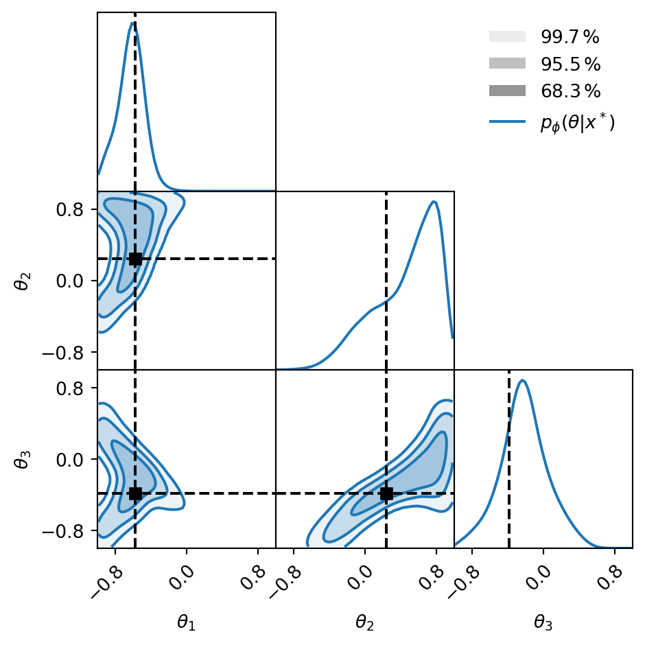
Weighted posterior

• NPE
• Weighted NPE
• Nested sampling

Outliers and effective sample size

The effective sample size is

\[ n _{\text{eff}} = \frac{(\sum_i w_i)^2}{\sum_i w_i^2}\,. \]

If \(q(\theta | d) = p(\theta| d)\), this is the number of samples. The sample efficiency is

\[ \epsilon = \frac{n _{\text{eff}}}{N}\in \left[ \frac{1}{N}, 1 \right]\,. \]

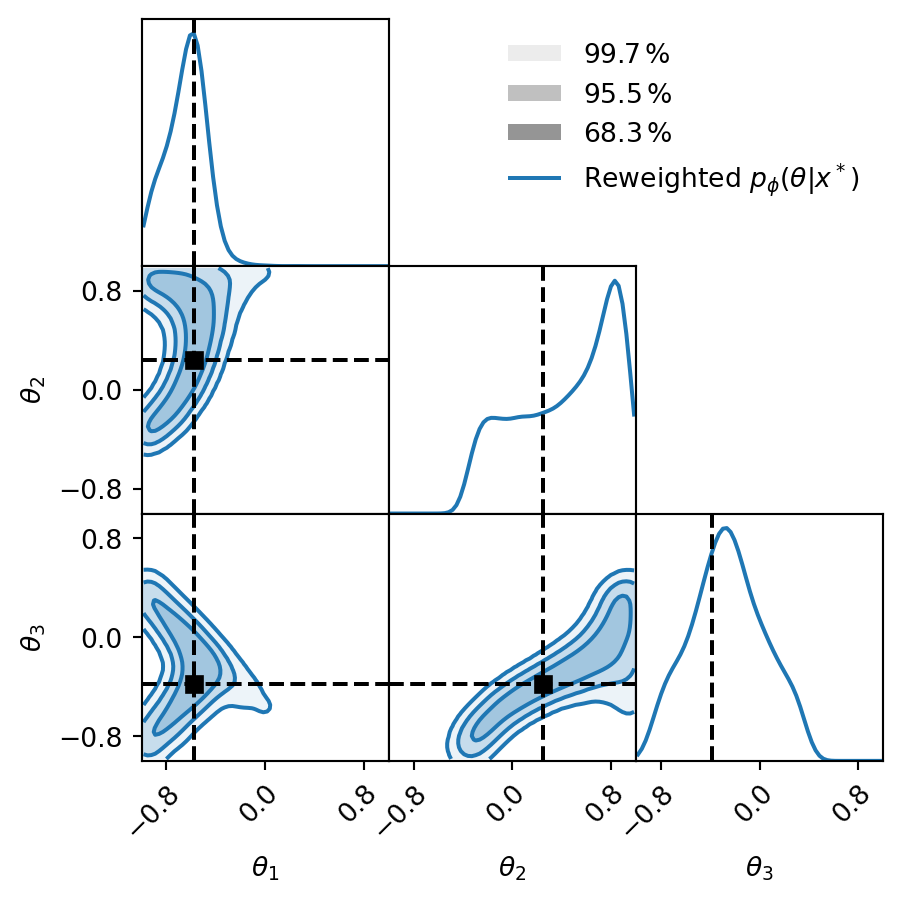
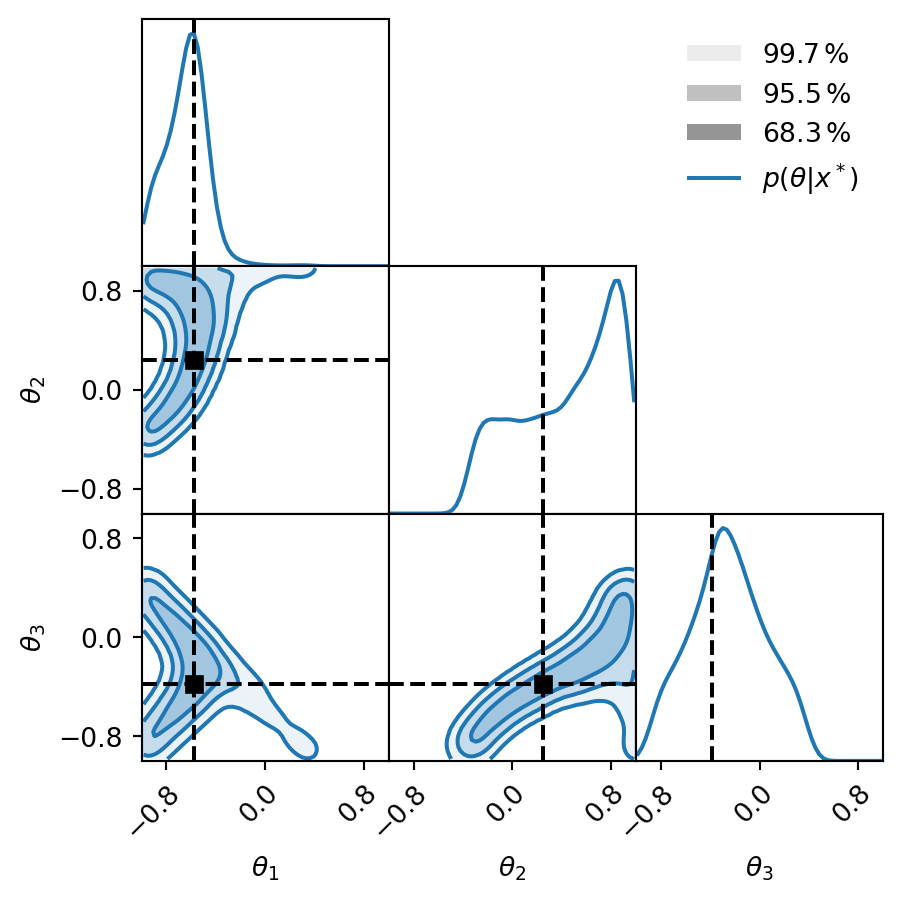
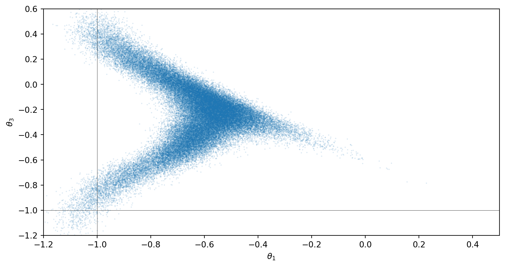
Weighted samples comparison

• NPE
• Weighted NPE

Back to gravitational waves

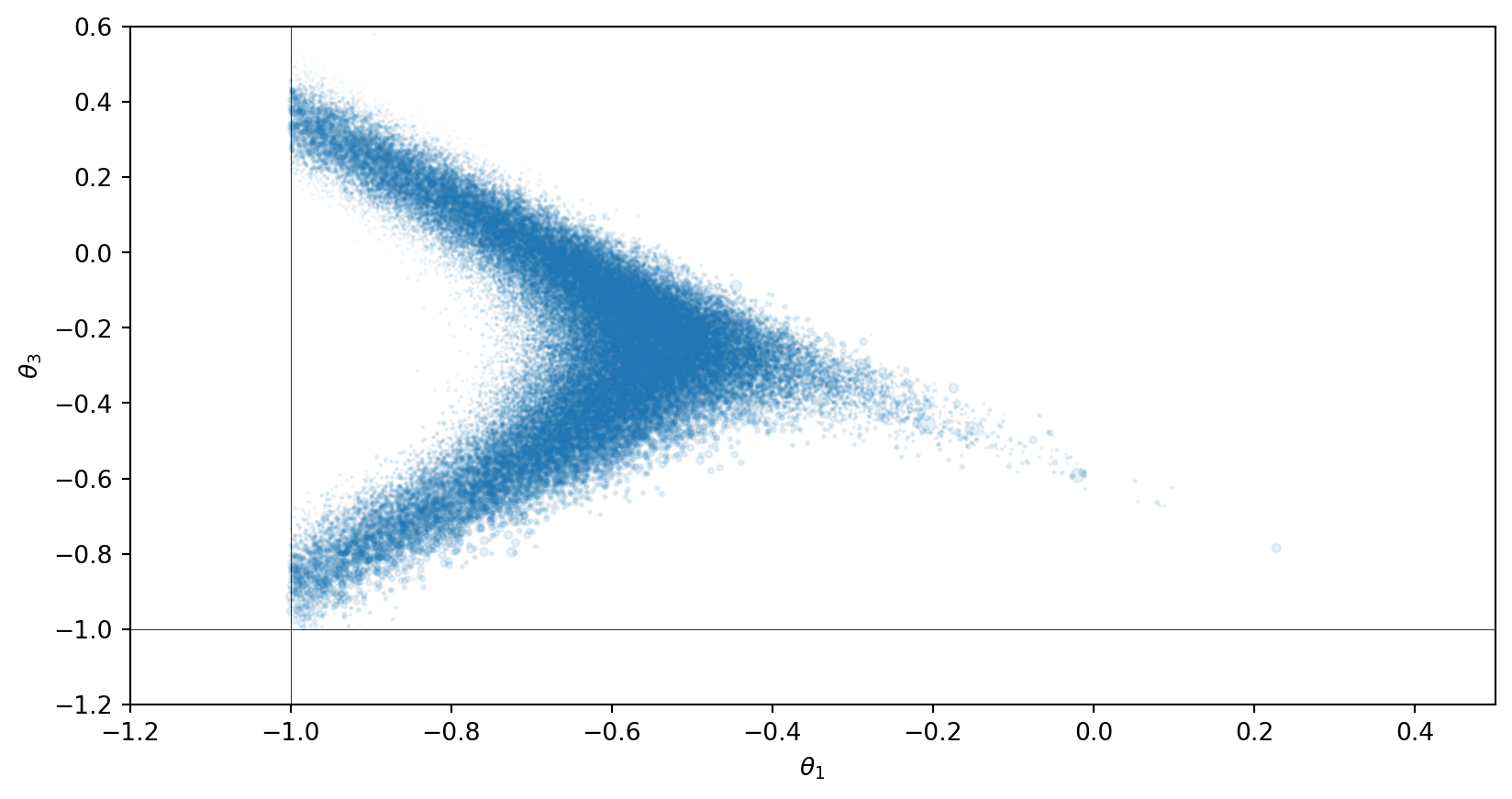
The arrival time problem

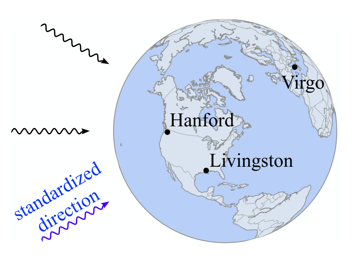
Standardization of the arrival direction (Dax et al. 2023).

Realistic loss function

It includes variation of the noise spectral density and Group-Equivariant NPE (Dax et al. 2023):

\[ \begin{aligned} L_{\text{GNPE}} = &\mathbb{E}_{\theta \sim \pi(\theta)} \\ &\mathbb{E}_{S_{n} \sim p(S_{n})} \\ &\mathbb{E}_{d \sim p(d|\theta)} \\ &\mathbb{E}_{ \delta t_{I} \sim \kappa (\delta t_{I})} [-\log q(\theta|d_{-t_{I}(\theta)-\delta t_{I}}, S_{n}, t_{I}(\theta) + \delta t_{I})]\,. \end{aligned} \]

Other approaches exist, such as heterodyning (Roulet et al. 2026).

Sample efficiency

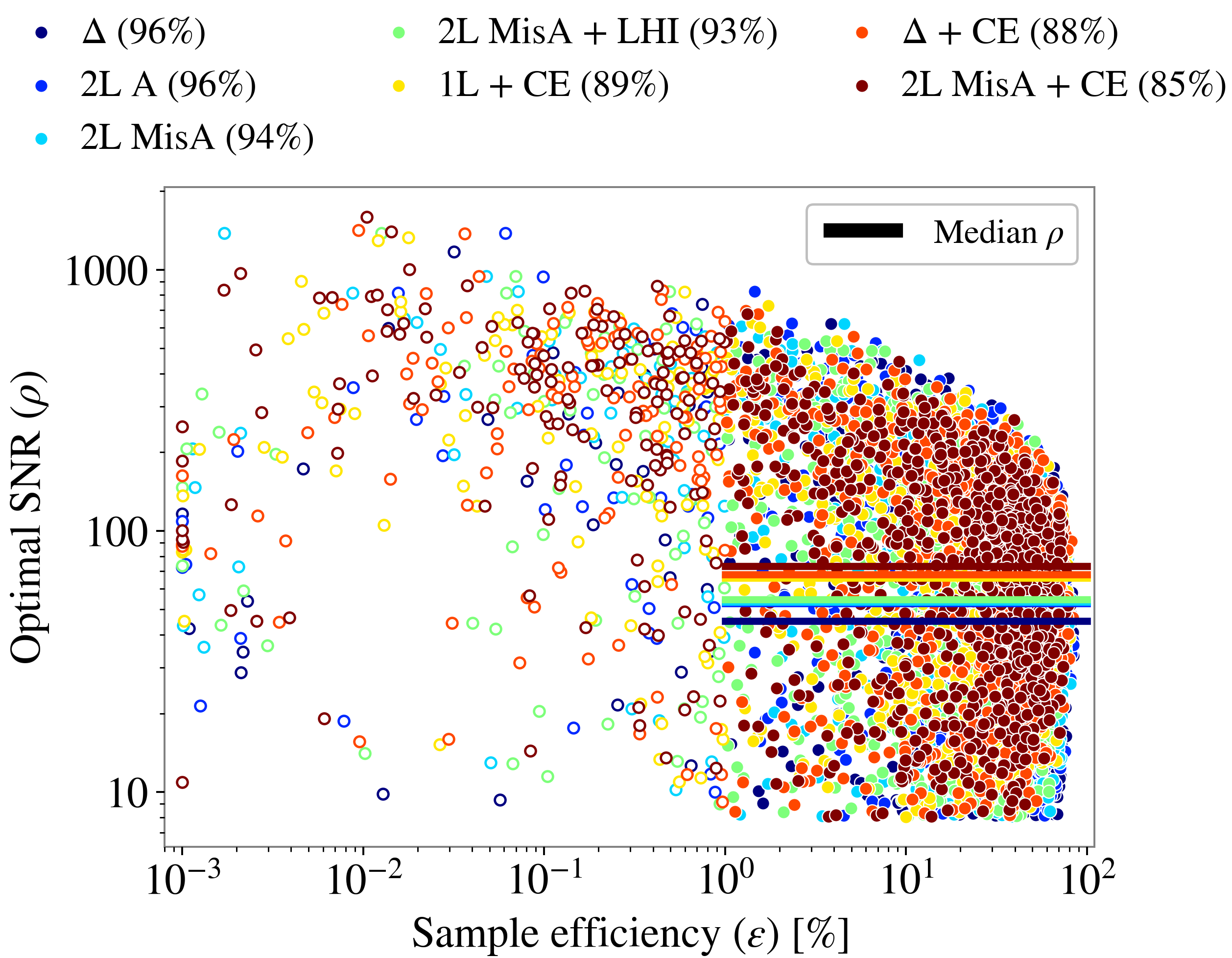
Sample efficiency as a function of SNR (Santoliquido et al. 2025).

On the flexibility of NPE

• All groups have so far have trained NPE on Gaussian noise.
• If we reweight with a Gaussian likelihood, it is pointless to train on anything other than Gaussian noise.
• There are efforts toward using SBI approaches other than NPE to handle non-Gaussian noise, e.g. Emma & Ashton (2026).

What do we want to know about gravitational wave sources?

Let’s chat!

• where do binaries of black holes come from?
• does General Relativity accurately describe them?
• how do neutron stars behave?
• how does the Universe look on a large scale?
• …

References

Abac AG, Abouelfettouh I, Acernese F, Ackley K, Adamcewicz C, et al. 2025. Phys. Rev. Lett. 135(11):111403

Dax M, Green SR, Gair J, Deistler M, Schölkopf B, Macke JH. 2023. Group equivariant neural posterior estimation. http://arxiv.org/abs/2111.13139

Dax M, Green SR, Gair J, Macke JH, Buonanno A, Schölkopf B. 2021. Phys. Rev. Lett. 127(24):241103

Emma M, Ashton G. 2026. RNLE: Residual neural likelihood estimation and its application to gravitational-wave astronomy. http://arxiv.org/abs/2601.13857

Liang B, Wang H. 2025. Astronomical Techniques and Instruments. 2(0):1–18

Papamakarios G, Murray I. 2016. Fast \epsilon -free Inference of Simulation Models with Bayesian Conditional Density Estimation

Powell J. 2018. Classical and Quantum Gravity. 35(15):155017

Roulet J, Crisostomi M, Thomas LM, Chatziioannou K. 2026. Labrador: A domain-optimized machine-learning tool for gravitational wave inference. http://arxiv.org/abs/2604.08897

Santoliquido F, Tissino J, Dupletsa U, Branchesi M, Harms J. 2025. Comparing next-generation detector configurations for high-redshift gravitational wave sources with neural posterior estimation. http://arxiv.org/abs/2512.20699